
| Home | Sources Directory | News Releases | Calendar | Articles | | Contact | |
Heritability

Heritability is the proportion of phenotypic variation in a population that is attributable to genetic variation among individuals. Phenotypic variation among individuals may be due to genetic and/or environmental factors. Heritability analyses estimate the relative contributions of differences in genetic and non-genetic factors to the total phenotypic variance in a population.
Pay close attention to the variation part of "phenotypic variation": if a trait has a heritability of 0.5, it means that the phenotypic variation is 50% due to genetic variation. It does not imply that the trait is 50% caused by genetics.
Heritability is also specific to a particular population in a particular environment.
Contents |
[edit] Overview

Rather than look at all the traits of an organism, heritability focuses on the differences between multiple organisms for a single trait. Because heritability is concerned with variance, it is necessarily a description of a certain population - not an individual.
A population of asians would contain individuals with genetics that code only for black hair. In this case, heritability is of course 0, since there is no variance in hair colour to analyse. But suppose some individuals dyed their hair and increased the population's variance in hair colours. Although now there are some differences in hair colour, theoretically heritability would still be 0 (i.e. 0% of the variance is due to differences in genetics).

Oppositely, imagine a population of mixed races where hair dye is forbidden. Now there is again variance in hair colour, but this time heritability is 1 (i.e. 100% of the variance is due to differences in genetics). Of course, that would be assuming that our population's hair colours truly have nothing to do with environmental factors (like amount of sunlight). In practice, heritability is not that simple; environment and genetics interact.
[edit] Definition

Consider a statistical model for describing some particular phenotype:[1]
- Phenotype (P) = Genotype (G) + Environment (E).
Considering variances (Var), this becomes:
- Var(P) = Var(G) + Var(E) + 2 Cov(G,E).
In planned experiments, we can often take Cov(G,E) = 0. Heritability is then defined as:
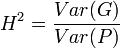 .
.
The parameter H2 is the broad-sense heritability and reflects all possible genetic contributions to a population's phenotypic variance. Included are effects due to allelic variation (additive variance), dominance variation, epistatic (multi-genic) interactions, and maternal and paternal effects, where individuals are directly affected by their parents' phenotype (such as with milk production in mammals).
These additional terms can be included in genetic models. For example, the simplest genetic model involves a single locus with two alleles that affect some quantitative phenotype, as shown by + in Figure 1. We can calculate the linear regression of phenotype on the number of B alleles (0, 1, or 2), which is shown as the Linear Effect line. For any genotype, BiBj, the expected phenotype can then be written as the sum of the overall mean, a linear effect, and a dominance deviation:
- Pij = î� + î�i + î�j + dij = Population mean + Additive Effect (aij = î�i + î�j) + Dominance Deviation (dij).
The additive genetic variance is the weighted average of the squares of the additive effects:

where f(bb)abb + f(Bb)aBb + f(BB)aBB = 0.
There is a similar relationship for variance of dominance deviations:

where f(bb)dbb + f(Bb)dBb + f(BB)dBB = 0.
Narrow-sense heritability is defined as

and quantifies only the portion of the phenotypic variation that is additive (allelic) by nature (note upper case H2 for broad sense, lower case h2 for narrow sense). When interested in improving livestock via artificial selection, for example, knowing the narrow-sense heritability of the trait of interest will allow predicting how much the mean of the trait will increase in the next generation as a function of how much the mean of the selected parents differs from the mean of the population from which the selected parents were chosen. The observed response to selection leads to an estimate of the narrow-sense heritability (called realized heritability).
[edit] Estimating heritability
Estimating heritability is not a simple process, since only P can be observed or measured directly. Measuring the genetic and environmental variance requires various sophisticated statistical methods. These methods give better estimates when using data from closely related individuals - such as brothers, sisters, parents and offspring, rather than from more distantly related ones. The standard error for heritability estimates is generally very poor unless the dataset is large.

In non-human populations it is often possible to collect information in a controlled way. For example, among farm animals it is easy to arrange for a bull to produce offspring from a large number of cows. Due to ethical concerns, such a degree of experimental control is impossible when gathering human data.
As a result, studies of human heritability sometimes contrast identical twins who have been separated early in life and raised in different environments (see for example Fig. 2). Such individuals have identical genotypes and can be used to separate the effects of genotype and environment.
Twin studies entail problems of their own, such as: independently raised twins shared a common prenatal environment; they may have undergone intrauterine competition; the mother may be more physically stressed (less nutrients); and twins reared apart are difficult to find, and may reflect certain types of environments.
Heritability estimates are always relative to the genetic and environmental factors in the population, and are not absolute measurements of the contribution of genetic and environmental factors to a phenotype. Heritability estimates reflect the amount of variation in genotypic effects compared to variation in environmental effects.
Heritability can be made larger by diversifying the genetic background, e.g., by using only very outbred individuals (which increases the Variance(G)) and/or by minimizing environmental effects (which decreases the Variance(E)). Smaller heritability, on the other hand, can be generated by using inbred individuals (which decreases the Variance(G)) or individuals reared in very diverse environments (which increases the Variance(E)). Due to such effects, different populations of a species might have different heritabilities even for the same trait.
In observational studies G and E may be correlated, giving rise to gene environment correlation. Depending on the methods used to estimate heritability, correlations between genetic factors and shared or non-shared environments may or may not be included in the total heritability estimate. [2]
Because of the contextual nature of measured heritabilities, paradoxes often arise. For example, the heritability of a trait could be near 100% in one study and close to zero in another. In one study, e.g., a group of unrelated army recruits may be given identical training and nutrition and then their muscular strength may be measured.
The variation in strength observed after the (identical) training will translate into a high heritability estimate. In another study, whose purpose might be to assess the efficacy of various workout regimes or nutritional programs, study subjects may be first chosen to match each other as closely as possible in prior physical characteristics before some of them are put onto Program A and others onto Program B, and this will lead to a low heritability estimate.
Heritability estimates are often misinterpreted. Heritability refers to the proportion of variation between individuals in a population that is influenced by genetic factors. Heritability describes the population, not individuals within that population. For example, It is incorrect to say that since the heritability of a personality trait is about .6, that means that 60% of your personality is inherited from your parents and 40% comes from the environment.
The heritability estimate changes according to the genetic and environmental variability present in the population. In studies of genetically identical inbred animals, all traits have zero heritability. Heritability estimates can be much higher in outbred (genetically variable) populations under very homogeneous environments.
A highly genetically loaded trait (such as eye color) still assumes environmental input within normal limits (a certain range of temperature, oxygen in the atmosphere, etc.). A more useful distinction than "nature vs. nurture" is "obligate vs. facultative" -- under typical environmental ranges, what traits are more "obligate" (e.g., the nose -- everyone has a nose) or more "facultative" (sensitive to environmental variations, such as specific language learned during infancy). Another useful distinction is between traits that are likely to be adaptations (such as the nose) vs. those that are byproducts of adaptations (such the white color of bones), or are due to random variation (non-adaptive variation in, say, nose shape or size).
[edit] Estimation methods
There are essentially two schools of thought regarding estimation of heritability.
One school of thought was developed by Sewall Wright at The University of Chicago, and further popularized by C. C. Li (University of Chicago) and J. L. Lush (Iowa State University). It is based on the analysis of correlations and, by extension, regression. Path Analysis was developed by Sewall Wright as a way of estimating heritability.
The second was originally developed by R. A. Fisher and expanded at The University of Edinburgh, Iowa State University, and North Carolina State University, as well as other schools. It is based on the analysis of variance of breeding studies, using the intraclass correlation of relatives. Various methods of estimating components of variance (and, hence, heritability) from ANOVA are used in these analyses.
[edit] Regression/correlation methods of estimation
The first school of estimation uses regression and correlation to estimate heritability.
[edit] Selection experiments

Calculating the strength of selection, S (the difference in mean trait between the population as a whole and the selected parents of the next generation, also called the selection differential [3]) and response to selection R (the difference in offspring and whole parental generation mean trait) in an artificial selection experiment will allow calculation of realized heritability as the response to selection relative to the strength of selection, h2=R/S as in Fig. 3.
[edit] Comparison of close relatives
In the comparison of relatives, we find that in general,
 where r can be thought of as the coefficient of relatedness, b is the coefficient of regression and t the coefficient of correlation.
[edit] Parent-offspring regression

Heritability may be estimated by comparing parent and offspring traits (as In Fig. 4). The slope of the line (0.57) approximates the heritability of the trait when offspring values are regressed against the average trait in the parents. If only one parent's value is used then heritability is twice the slope. (note that this is the source of the term "regression", since the offspring values always tend to regress to the mean value for the population, i.e., the slope is always less than one).
[edit] Full-sib comparison
Full-sib designs compare phenotypic traits of siblings that share a mother and a father with other sibling groups. The estimate of the sibling phenotypic correlation is an index on familiality which is equal to half the additive genetic variance plus the common environment variance when there is only additive gene action.
| This section requires expansion. |
[edit] Half-sib comparison
Half-sib designs compare phenotypic traits of siblings that share one parent with other sibling groups.
| This section requires expansion. |
[edit] Twin studies

Heritability for traits in humans is most frequently estimated by comparing resemblances between twins (Fig. 2 & 5). Identical twins (MZ twins), on average, are twice as genetically similar as fraternal twins (DZ twins) and so heritability is approximately twice the difference in correlation between MZ and DZ twins, i.e. Falconer's formula h2=2(r(MZ)-r(DZ)).
The effect of shared environment, c2, contributes to similarity between siblings due to the commonality of the environment they are raised in. Shared environment is approximated by the DZ correlation minus half heritability, which is the degree to which DZ twins share the same genes, c2=DZ-1/2h2. Unique environmental variance, e2, reflects the degree to which identical twins raised together are dissimilar, e2=1-r(MZ).
The methodology of the classical twin study has been criticized, but some of these criticisms do not take into account the methodological innovations and refinements described above.
[edit] Large, complex pedigrees
| This section requires expansion. |
[edit] Analysis of variance methods of estimation
The second set of methods of estimation of heritability involves ANOVA and estimation of variance components.
[edit] Basic model
We use the basic discussion of Kempthorne (1957 [1969]). Considering only the most basic of genetic models, we can look at the quantitative contribution of a single locus with genotype Gi as
yi = î� + gi + e
where
gi is the effect of genotype Gi
and e is the environmental effect.
Consider an experiment with a group of sires and their progeny from random dams. Since the progeny get half of their genes from the father and half from their (random) mother, the progeny equation is

[edit] Intraclass correlations
Consider the experiment above. We have two groups of progeny we can compare. The first is comparing the various progeny for an individual sire (called within sire group). The variance will include terms for genetic variance (since they did not all get the same genotype) and environmental variance. This is thought of as an error term.
The second group of progeny are comparisons of means of half sibs with each other (called among sire group). In addition to the error term as in the within sire groups, we have an addition term due to the differences among different means of half sibs. The intraclass correlation is
 ,
,
since environmental effects are independent of each other.
[edit] The ANOVA
In an experiment with n sires and r progeny per sire, we can calculate the following ANOVA, using Vg as the genetic variance and Ve as the environmental variance:
| Source | d.f. | Mean Square | Expected Mean Square |
|---|---|---|---|
| Among sire groups | n ' 1 | S | 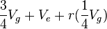 |
| Within sire groups | n(r ' 1) | W |  |
The  term is the intraclass correlation among half sibs. We can easily calculate
  . The Expected Mean Square is calculated from the relationship of the individuals (progeny within a sire are all half-sibs, for example), and an understanding of intraclass correlations.
[edit] Model with additive and dominance terms
For a model with additive and dominance terms, but not others, the equation for a single locus is
- yij = î� + î�i + î�j + dij + e,
where
î�i is the additive effect of the ith allele, î�j is the additive effect of the jth allele, dij is the dominance deviation for the ijth genotype, and e is the environment.
Experiments can be run with a similar setup to the one given in Table 1. Using different relationship groups, we can evaluate different intraclass correlations. Using Va as the additive genetic variance and Vd as the dominance deviation variance, intraclass correlations become linear functions of these parameters. In general,
- Intraclass correlation = rVa + î�Vd,
where r and î� are found as
r = P[ alleles drawn at random from the relationship pair are identical by descent], and
î� = P[ genotypes drawn at random from the relationship pair are identical by descent].
Some common relationships and their coefficients are given in Table 2.
| Relationship | r | î� |
|---|---|---|
| Identical Twins | 1 | 1 |
| Parent-Offspring |  |
0 |
| Half Siblings |  |
0 |
| Full Siblings | |
|
| First Cousins |  |
0 |
| Double First Cousins | |
 |
[edit] Larger models
When a large, complex pedigree is available for estimating heritability, the most efficient use of the data is in a restricted maximum likelihood (REML) model. The raw data will usually have three or more datapoints for each individual: a code for the sire, a code for the dam and one or several trait values. Different trait values may be for different traits or for different timepoints of measurement.
The currently popular methodology relies on high degrees of certainty over the identities of the sire and dam; it is not common to treat the sire identity probabilistically. This is not usually a problem, since the methodology is rarely applied to wild populations (although it has been used for several wild ungulate and bird populations), and sires are invariably known with a very high degree of certainty in breeding programmes. There are also algorithms that account for uncertain paternity.
The pedigrees can be viewed using programs such as Pedigree Viewer [1], and analysed with programs such as ASReml, VCE [2], WOMBAT [3] or BLUPF90 family's programs [4]
[edit] Response to Selection
In selective breeding of plants and animals, the expected response to selection can be estimated by the following equation:[4]
R = h2S
In this equation, the Response to Selection (R) is defined as the realized average difference between the parent generation and the next generation. The Selection Differential (S) is defined as the average difference between the parent generation and the selected parents.
For example, imagine that a plant breeder is involved in a selective breeding project with the aim of increasing the number of kernels per ear of corn. For the sake of argument, let us assume that the average ear of corn in the parent generation has 100 kernels. Let us also assume that the selected parents produce corn with an average of 120 kernels per ear. If h2 equals 0.5, then the next generation will produce corn with an average of 0.5(120-100) = 10 additional kernels per ear. Therefore, the total number of kernels per ear of corn will equal, on average, 110.
[edit] See also
[edit] References
[edit] Notes
- ^ The presentation here roughly follows Kempthorne (1957)
- ^ Cattell RB (1960). "The multiple abstract variance analysis equations and solutions: for nature'nurture research on continuous variables". Psychol Rev 67: 353'372. doi:10.1037/h0043487. PMID 13691636.
- ^ Kempthorne (1957), page 507; or Falconer (1960), page 191, for example.
- ^ Plomin, R., DeFries, J. C., & McClearn, G. E. (1990). Behavioral genetics. New York: Freeman.
[edit] Further reading
- Falconer, D. S. & Mackay TFC (1996). Introduction to Quantitative Genetics. Fourth edition. Addison Wesley Longman, Harlow, Essex, UK
- Gillespie, G. H. (1997). Population Genetics: A Concise Guide. Johns Hopkins University Press.
- Joseph, J. (2004). The Gene Illusion: Genetic Research in Psychiatry and Psychology Under the Microscope. New York: Algora. (2003 United Kingdom Edition by PCCS Books) (Chapter 5 contains a critique of the heritability concept)
- Joseph, J. (2006). The Missing Gene: Psychiatry, Heredity, and the Fruitless Search for Genes. New York: Algora.
- Kempthorne, O (1957 [1969]) An Introduction to Genetic Statistics. John Wiley. Reprinted, 1969 by Iowa State University Press.
- Lynch, M. & Walsh, B. 1997. Genetics and Analysis of Quantitative Traits. Sinauer Associates. ISBN 0-87893-481-2.
- Malécot, G. 1948. Les Mathématiques de l'Hérédité. Masson, Paris.
- Wahlsten, D. (1994) The intelligence of heritability. Canadian Psychology 35, 244-258.
[edit] External links
- Stanford Encyclopedia of Philosophy entry on Heredity and Heritability
- Quantitative Genetics Resources website, including the two volume book by Lynch and Walsh. Free access
|
||||||||||

|
||||||||||||||||||||||||||
|
SOURCES.COM is an online portal and directory for journalists, news media, researchers and anyone seeking experts, spokespersons, and reliable information resources. Use SOURCES.COM to find experts, media contacts, news releases, background information, scientists, officials, speakers, newsmakers, spokespeople, talk show guests, story ideas, research studies, databases, universities, associations and NGOs, businesses, government spokespeople. Indexing and search applications by Ulli Diemer and Chris DeFreitas.
For information about being included in SOURCES as a expert or spokesperson see the FAQ . For partnerships, content and applications, and domain name opportunities contact us.